Stretched-Grid Simulation: Eastern US

This tutorial walks you through setting up and running a stretched-grid simulation for ozone in the eastern US. The grid parameters for this tutorial are

Parameter	Value
Stretch-factor	3.6
Cubed-sphere size	C60
Target latitude	37° N
Target longitude	275° E

These parameters were choosen so that the target face covered the eastern US. Some back-of-the-envelope resolution calculations are

\[\mathrm{average\ resolution\ of\ target\ face = R_{tf} \approx \frac{10000\ km}{N \times S} = 46\ km}\]

and

\[\mathrm{coarsest\ resolution\ in\ target\ face\ (at\ the\ center) \approx R_{tf} \times 1.2 = 56\ km }\]

and

\[\mathrm{finest\ resolution\ in\ target\ face\ (at\ the\ edges) \approx R_{tf} \div 1.2 = 39\ km }\]

and

\[\mathrm{coarsest\ resolution\ globally\ (at\ target\ antipode) \approx R_{tf} \times S^2 \times 1.2 = 720\ km }\]

where \(\mathrm{N}\) is the cubed-sphere size and \(\mathrm{S}\) is the stretch-factor. The actual value of these, calculated from the grid-box areas, are 46 km, 51 km, 42 km, and 664 km respectively.

Note

This tutorial uses a relatively large stretch-factor. A smaller stretch-factor, like 2.0, would have a refinement that more broad, and the range resolutions would be smaller.

Tutorial prerequisites

Before continuing with the tutorial:

• You need to be able to run GCHP simulations

• You need to install gcpy >= 1.0.0, and cartopy >= 0.19

• You need emissions data and MERRA2 data for July 2019

Create a new run directory. This run directory should be use full chemistry with standard simulation options, and use MERRA2 meteorology. Make the following modifications to runConfig.sh:

• Change the simulation’s start time to "20190701 000000"

• Change the simulation’s end time to "20190708 000000"

• Change the simulation’s duration to "00000007 000000"

• Change timeAvg_freq to "240000" (daily diagnostics)

• Change timeAvg_dur to "240000" (daily diagnostics)

• Update the compute resources as you like. This simulation’s computational demands are about \(1.5\times\) that of a C48 or 2°x2.5° simulation.

Note

I chose to use 30 cores on 1 node, and the simulation took 7 hours to run. For comparison, I also ran the simulation on 180 cores across 6 nodes, and that took about 2 hours.

Update gchp.local.run so nCores matches your setting in runConfig.sh. Now you are ready to continue with the tutorial. The rest of the tutorial assume that your current working directory is your run directory.

Create your restart file

First, create a restart file for the simulation. GCHP ingests the restart file directly (no online regridding), so the first thing you need to do is regrid a restart file to your stretched-grid. You can regrid initial_GEOSChem_rst.c48_fullchem.nc with GCPy like so:

$ python -m gcpy.file_regrid                           \
     -i initial_GEOSChem_rst.c48_fullchem.nc           \
     --dim_format_in checkpoint                        \
     --dim_format_out checkpoint                       \
     --cs_res_out 60                                   \
     --sg_params_out 3.6 275 37                        \
     -o initial_GEOSChem_rst.EasternUS_SG_fullchem.nc

This creates initial_GEOSChem_rst.EasternUS_SG_fullchem.nc, which is the new restart file for your simulation.

Note

This command takes about a minute to run. If you regridding a large restart file (e.g., C180) it may take significantly longer.

Update runConfig.sh

Make the following updates to runConfig.sh:

• Change INITIAL_RESTART to use initial_GEOSChem_rst.EasternUS_SG_fullchem.nc

• Change CS_RES to 60

• Change STRETCH_GRID to ON

• Change STRETCH_FACTOR to 3.6

• Change TARGET_LAT to 37.0

• Change TARGET_LON to 275.0

Execute runConfig.sh to apply the updates to the various configuration files:

$ ./runConfig.sh

Run GCHP

Run GCHP:

$ ./gchp.local.run

Plot the output

Append grid-box corners:

$ python -m gcpy.append_grid_corners \
     --sg_params 3.6 275 37 \
     OutputDir/GCHP.SpeciesConc.20190707_1200z.nc4

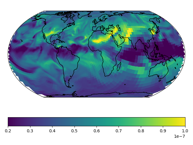
Plot ozone at model level 22:

import matplotlib.pyplot as plt
import cartopy.crs as ccrs
import xarray as xr

# Load 24-hr average concentrations for 2019-07-07
ds = xr.open_dataset('GCHP.SpeciesConc.20190707_1200z.nc4')

# Get Ozone at level 22
ozone_data = ds['SpeciesConc_O3'].isel(time=0, lev=22).squeeze()

# Setup axes
ax = plt.axes(projection=ccrs.EqualEarth())
ax.set_global()
ax.coastlines()

# Plot data on each face
for face_idx in range(6):
    x = ds.corner_lons.isel(nf=face_idx)
    y = ds.corner_lats.isel(nf=face_idx)
    v = ozone_data.isel(nf=face_idx)
    pcm = plt.pcolormesh(
        x, y, v,
        transform=ccrs.PlateCarree(),
        vmin=20e-9, vmax=100e-9
    )

plt.colorbar(pcm, orientation='horizontal')
plt.show()