Plotting GCHP Output
Panoply
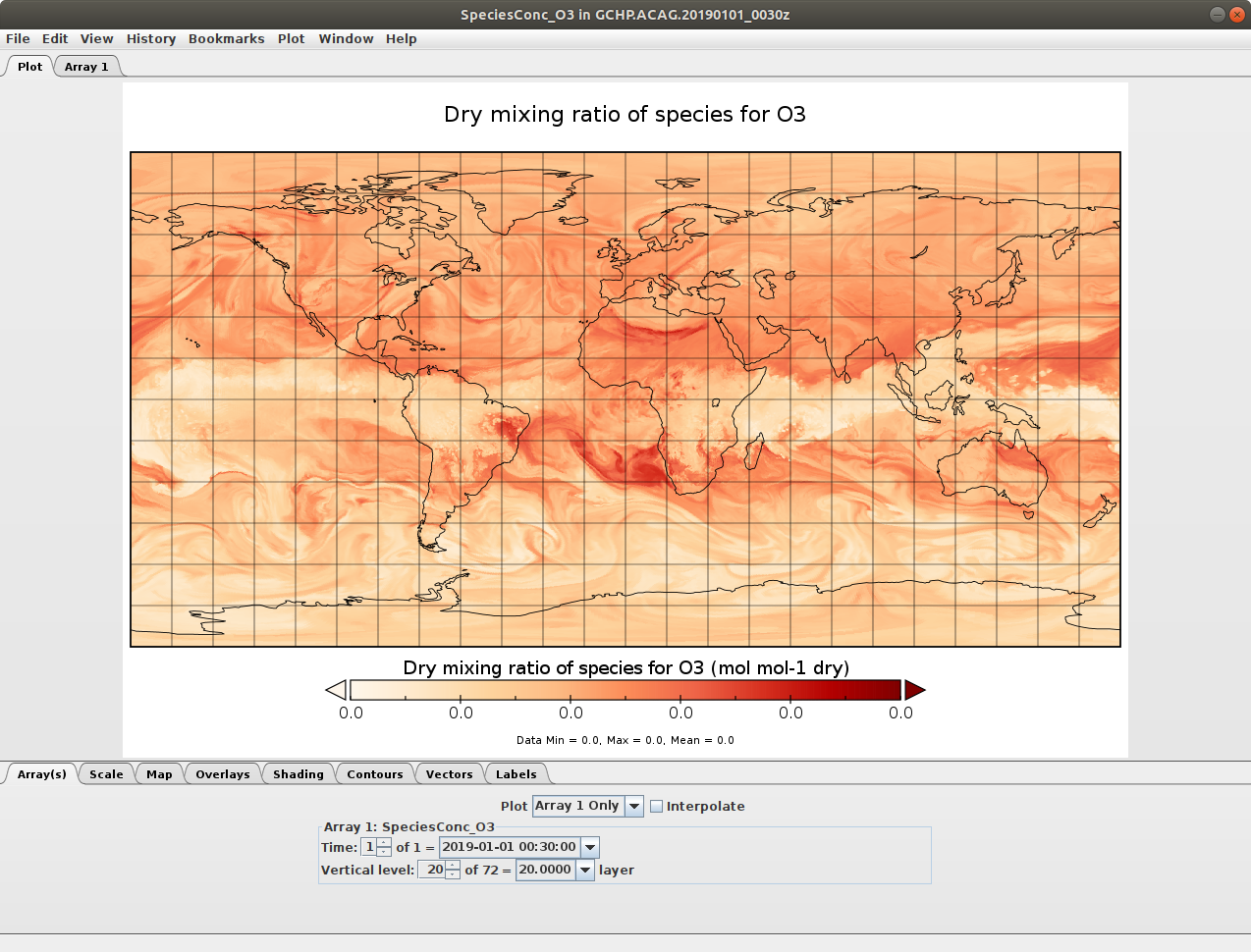
Panoply is useful for quick and easy viewing of GCHP output. Panoply is a grahpical program for plotting geo-referenced data like GCHP’s output. It is an intuitive program and it is easy to set up.
You can read more about Panoply, including how to install it, here.
- Some suggestions
If you can mount your cluster’s filesystem as a Network File System (NFS) on your local machine, you can install Panoply on your local machine and view your GCHP data through the NFS.
If your cluster supports a graphical interface, you could install Panoply (administrative priviledges not necessary, provided Java is installed) yourself.
Alternatively, you could install Panoply on your local machine and use scp or similar to transfer files back and forth when you want to view them.
Note
To get rid of the missing value bands along face edges, uncheck ‘Interpolate’ (turn interpolation off) in the Array(s) tab.
Python
To plot GCHP data with Python you will need the following libraries:
cartopy >= 0.19 (0.18 won’t work – see cartopy#1622)
xarray
netcdf4
If you use conda you can install these packages like so
$ conda activate your-environment-name
$ conda install cartopy>=0.19 xarray netcdf4 -c conda-forge
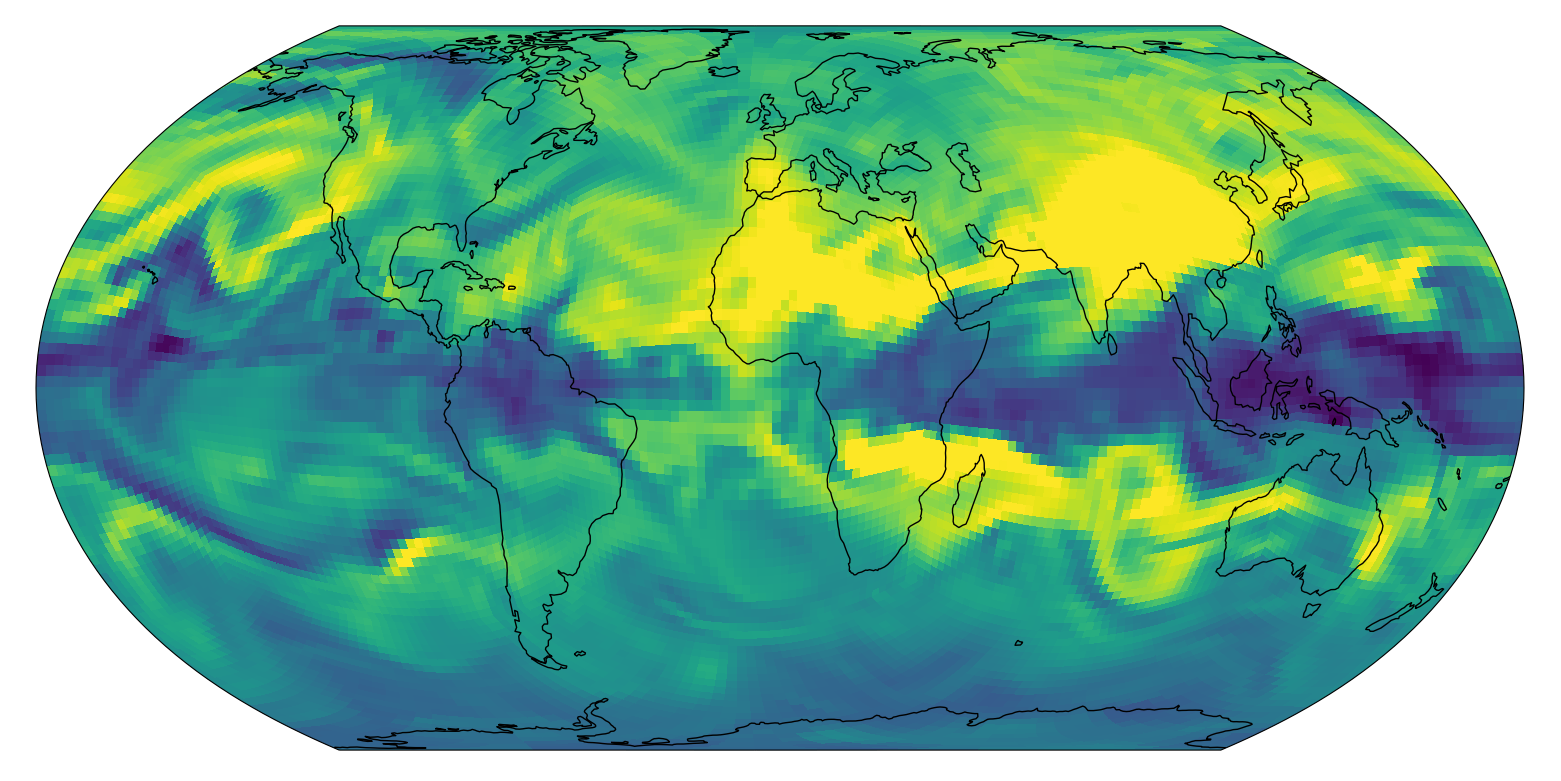
Here is a basic example of plotting cubed-sphere data:
Sample data:
GCHP.SpeciesConc.20210508_0000z.nc4
import matplotlib.pyplot as plt
import cartopy.crs as ccrs  # cartopy must be >=0.19
import xarray as xr

ds = xr.open_dataset('GCHP.SpeciesConc.20210508_0000z.nc4')  # see note below for download instructions

plt.figure()
ax = plt.axes(projection=ccrs.EqualEarth())
ax.coastlines()
ax.set_global()

norm = plt.Normalize(1e-8, 7e-8)

for face in range(6):
    x = ds.corner_lons.isel(nf=face)
    y = ds.corner_lats.isel(nf=face)
    v = ds.SpeciesConc_O3.isel(time=0, lev=23, nf=face)
    ax.pcolormesh(x, y, v, norm=norm, transform=ccrs.PlateCarree())

plt.show()
Note
The grid-box corners should be used with pcolormesh() because the grid-boxes are not regular (it’s a curvilinear grid).
This is why we use corner_lats and corner_lons in the example above.